This article is for personal use to roughly review basic oriented bounding box algorithms and practice JAX coding.
What is Oriented Minimum Bounding Box?
According to the Wikipedia, we get the following definitions about different bounding boxes.
1. Minimum bouding box
In geometry, the minimum or smallest bounding or enclosing box for a point set S in N dimensions is the box with the smallest measure (area, volume, or hypervolume in higher dimensions) within which all the points lie.
2. Axis-aligned minimum bounding box
The axis-aligned minimum bounding box (or AABB) for a given point set is its minimum bounding box subject to the constraint that the edges of the box are parallel to the (Cartesian) coordinate axes.
3. Arbitrarily oriented minimum bounding box
The arbitrarily oriented minimum bounding box (or OBB) is the minimum bounding box, calculated subject to no constraints as to the orientation of the result.

As you can see in the drawing, AABB is constrained to the coordinate axis of the image, whereas OBB is free of that. Usually, AABB is used to speed up the collision check of the physics simulation, skipping the complex collision checking algorithms for objects that AABBs do not intersect. In other words, OBB is used for creating a collision shape for objects to speed up the collision check itself.
To get AABB for the mesh, you just have to compute the minimum and maximum values of all points in the mesh for each coordinate axis, which does not require expensive computation. However, that is not the case for OBB that has bigger or equal dimension of three. Therefore, in this article, we review algorithms for OBB and try to find a simple implementation for it.
One important note before we get into the algorithms is the fact that the minimum bouding box for $N$ points is the same as the minimum bouding box for the convex hull of those $N$ points, which has $n$ points that $n$ is a lot smaller than $N$. Most of the time, convex hull algorithms ($O(n log(h))$) are faster than minimum bouding box algorithms ($O(n^3)$). Therefore, most of the minimum bounding box algorithms reduce the number of points by using a convex hull algorithm first so that the order of computation is $O(Nlog(h)+O(n^3)$.
1. Baseline: Joseph O'Rourke's algorithm ($O(n^3)$)
This baseline is well documented in the Wikipedia. It is based on two lemmas.
- There must exist two neighbouring faces of the smallest-volume enclosing box which both contain an edge of the convex hull of the point set. This criterion is satisfied by a single convex hull edge collinear with an edge of the box, or by two distinct hull edges lying in adjacent box faces.
- The other four faces need only contain a point of the convex hull. Again, the points which they contain need not be distinct: a single hull point lying in the corner of the box already satisfies three of these four criteria.
Basically, it checks all three points that might share a face with OBB and calculates all possible OBB to return the minimum one. There are $(1+\epsilon)$-approximate algorithms to speed up this process, using grid and grid search. However, they are usually complicated to implement and require additional approximate information about the direction of OBB. Also, they are still slow to be used in the real world. Therefore, in a practical sense, people use heuristic approaches that are proven to be faster than O'Rourke's algorithm in most cases.
2. Heuristic: Principal Component Analysis (PCA)
Heuristic approaches try to find the direction of convex hull points, rotate the convex hull points according to it, and use the AABB algorithm to get the OBB. We know from college mathematics class that one way to get the direction of points in 3D space is to use PCA. If we set $\hat x=E(x)$ as a mean of $x$ values of points, $\hat y=E(y)$ as a mean of $y$ values of points, and $\hat z=E(z)$ as a mean of $z$ values of points, we get the following covariance matrix:
$$C=\begin{bmatrix} E(xx)-\hat x\hat x&E(xy)-\hat x\hat y&E(xz)-\hat x\hat z\\ E(yx)-\hat y\hat x&E(yy)-\hat y\hat y&E(yz)-\hat y\hat z\\ E(zx)-\hat z\hat x&E(zy)-\hat z\hat y&E(zz)-\hat z\hat z \end{bmatrix}$$
If normalized eigenvectors of the covariance matrix is $i$, $j$, and $k$, we get the rotation matrix
$$R=\begin{bmatrix}i_1&j_1&k_1\\ i_2&j_2&k_2\\ i_3&j_3&k_3\end{bmatrix}$$
Therefore, if we rotate the points using $R$, get AABB for the points, and rotate the AABB with $R^{-1}$, we can get the OBB of the original points. This method is pretty easy because we can get the covariance matrix and eigenvectors by simply using Python libraries like Numpy or Scipy. However, there is a downside to this method.

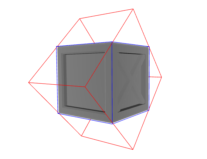
If the distribution of points of the mesh are symmetric and close to the sphere, the PCA method (red box) will not be able to capture the direction well like in the image above. Of course, there is a tradeoff between simplicity and accuracy, but there are a lot of times when this failure happens because many 3D mesh objects have very spherical distributions, meaning that they have symmetrical shapes on all axes.
3. Heuristic: Genetic algorithm
Many conventional programs use a genetic algorithm, which shows good robustness to local minima, to get both fast (<0.5s) and accurate OBB of the mesh. The below image shows the result of using a genetic algorithm called Matrix Adaptation Evolution Strategy (MAES) to find the rotation matrix.

Genetic algorithms are heuristic search algorithms that are usually used when the gradient of the cost function, which is the volume of the bounding box in our case, is not available for the optimization problem. The code for the cost function is written below.
import numpy as np

def rotation_matrix(a: float, b: float, r: float):
    # a,b,r are rotation angles in radians
    ca, sa = np.cos(a), np.sin(a)
    cb, sb = np.cos(b), np.sin(b)
    cr, sr = np.cos(r), np.sin(r)
    matrix = np.array(((cb*cr, sa*sb*cr-ca*sr, ca*sb*cr+sa*sr),
                       (cb*sr, sa*sb*sr+ca*cr, ca*sb*sr-sa*cr),
                       (-sb, sa*cb, ca*cb)))
    return matrix

def AABB_volume(mesh_vertices):
    # mesh_vertices (nx3 array of mesh vertices)
    x_length = max(mesh_vertices[:,0]) - min(mesh_vertices[:,0])
    y_length = max(mesh_vertices[:,1]) - min(mesh_vertices[:,1])
    z_length = max(mesh_vertices[:,2]) - min(mesh_vertices[:,2])
    return x_length*y_length*z_length

def cost_function(mesh_vertices):
    # mesh_vertices (nx3 array of mesh vertices)
    def foo(x):
        return AABB_volume((rotation_matrix(x[0],x[1],x[2])@mesh_vertices.T).T)
    return foo
You can simply use Python libraries like pypop or PyGAD for genetic algorithms. Or you can implement it by yourself, which is not that difficult and its method can be easily searched for. If you are looking for a blog for Python implementation, I recommend this link.
4. Heuristic: Differentiable computing
Even though the genetic algorithms are super fast and accurate, I wanted to look for a simpler yet accurate solution for OBB. Therefore, I came up with the idea of making the cost function differentiable. Normally, getting gradients of the cost function we use for a genetic algorithm is impossible or extremely difficult. However, if we use differentiable computing like JAX, we can easily get the gradients and use gradient descent methods to get OBB. The code is written below.
import jax
import jax.numpy as jnp
from jax import grad, jit
from jax.example_libraries import optimizers

def rotation_matrix(a, b, r):
    # a,b,r are rotation angles in radians
    ca, sa = jnp.cos(a), jnp.sin(a)
    cb, sb = jnp.cos(b), jnp.sin(b)
    cr, sr = jnp.cos(r), jnp.sin(r)
    matrix = jnp.array(((cb*cr, sa*sb*cr-ca*sr, ca*sb*cr+sa*sr),
                       (cb*sr, sa*sb*sr+ca*cr, ca*sb*sr-sa*cr),
                       (-sb, sa*cb, ca*cb)))
    return matrix

def AABB_volume(mesh_vertices):
    # mesh_vertices (nx3 array of mesh vertices)
    x_length = jnp.max(mesh_vertices[:,0]) - jnp.min(mesh_vertices[:,0])
    y_length = jnp.max(mesh_vertices[:,1]) - jnp.min(mesh_vertices[:,1])
    z_length = jnp.max(mesh_vertices[:,2]) - jnp.min(mesh_vertices[:,2])
    return x_length*y_length*z_length

def cost_function(mesh_vertices):
    # mesh_vertices (nx3 array of mesh vertices)
    def foo(x):
        return AABB_volume((rotation_matrix(x[0],x[1],x[2])@mesh_vertices.T).T)
    return foo

cost_f = cost_function(mesh_vertices)
derivative_fn = grad(cost_f)

# initialize the optimizer with arbitrary variables
initial_state = jnp.array([jnp.pi/4,jnp.pi/4,jnp.pi/4])
opt_init, opt_update, get_params = optimizers.adam(step_size=1e-2)
opt_state = opt_init(initial_state)

def learning_step(i, opt_state):
    grads = derivative_fn(get_params(opt_state))
    opt_state = opt_update(0, grads, opt_state)
    return opt_state

@jit
def learning():
    return get_params(jax.lax.fori_loop(0, 100, learning_step, opt_state))

final_state = learning()
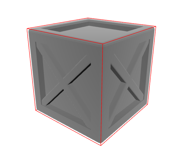
We can get a pretty good result with a differentiable computing method using Google Colab, like in the image below.

The downside of this method is that it takes some time to compile the JAX code, which is more than a second. However, if you are going to get OBB for multiple different meshes, you can further optimize and parallelize the code, which will give the edge to this method compared to the genetic algorithm method. Another thing you have to be careful about is that you have to use a good optimizer to avoid local minimas. Usually, Adam is a good optimizer you can use for most cases.
'Physics Simulation' 카테고리의 다른 글
| Collision Detection - Dynamic AABB Tree (0) | 2023.01.08 |
|---|---|
| Mesh to Signed Distance Function (0) | 2022.11.21 |
| Signed Distance Function Visualization (0) | 2022.11.03 |
| Oriented Minimum Bounding Volume for 3D Mesh (0) | 2022.10.19 |
| Visualization of Physics Simulation in Google Colab (0) | 2022.10.08 |